Diagnostics

PP creates extensive diagnostic output to provide the user with a comfortable way to verify the quality of the derived results. Focusing on human readability, the diagnostic output is in the form of a HTML website that is accessible with any web browser.

An example diagnostic output is provided here.

Overview

HTML Output

The diagnostic output for one specific data set can be accessed by opening the diagnostics.html website that is by default created in the respective data directory, e.g., using:

firefox diagnostics.html

Data presented in this website are all stored in a sub-directory named .diagnostics/ in the respective data directory (note that the dot prefix makes this a hidden directory).

LOG File

All tasks performed by PP are documented using Python’s logging system. The LOG file is linked from the diagnostics.html file (see top of the page). The LOG file can be used to check proper performance of the pipeline. Its main purpose is to simplify debbuging in case something went wrong. The LOG file is by default created in the respective data directory.

Diagnostics Details

The following sections discuss the output of a successful pipeline run in detail based on this example page.

Overview Information

The top of the diagnostics website lists the data directory, some general information like the telescope/instrument combination, as well as the total number of frames processed. The process LOG file (see above) is linked here, too.

All the frames considered in the process are listed in the Data Summary table, providing information on the date and time, target, filter, airmass, exposure time, and field of view. By default, the frame name links to a separate page with more information on that specific frame.

Registration

The first line of this section lists the astrometric catalog that was used in the registration and whether the registration was successfull, or not. The following table lists for each frame some diagnostics provided by SCAMP, including C:subscript:AS and C:subscript:XY that indicate the goodness of the frame’s rotation angle and scale, and the frame’s shift, respectively. \(\sigma\)_RA and \(\sigma\)_DEC provide a sense for positional uncertainties in arcsecs; \(\chi\)²_Reference and \(\chi\)²_Internal quantify the goodness of fit. For additional information on these parameters, please refer to the SCAMP manual. By default, the image filenames lead to a separate frame report page.

Instrumental Photometry

The optimum aperture size used by PP is determined using a curve-of-growth analysis. Details on how the optimum aperture was derived is provided in this section.

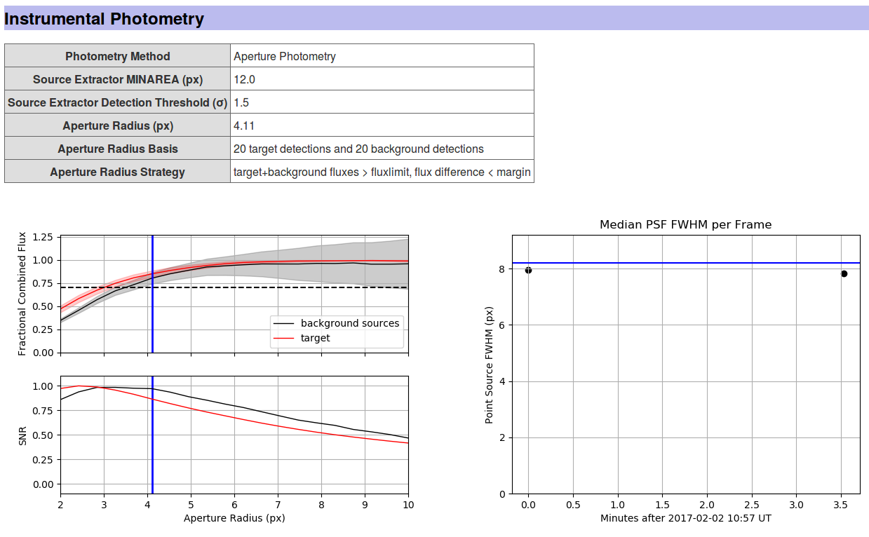
The left plot documents the curve-of-growth analysis. For a range of aperture sizes, the flux and SNR of both the target (red line) and the average over all background sources (black line) are determined. Note that both the flux and the SNR are fractional values - they are relative to the maximum flux (of either the target or the background stars) or the maximum SNR. In order to obtain reliable photometry, you want to include as much flux as possible but at the same time keep the aperture as small as possible, in order to minimize noise introduced by the background - this is reflected by the SNR’s peak (see, e.g, Howell’s Handbook of CCD Astronomy for a discussion). PP deliberately does not use the aperture radius that provides the highest SNR. The optimum aperture radius is required to include at least 70% of the both the target’s and background sources’ flux - at the same time, the fractional flux difference between the target and background sources has to be smaller than 5%. Both conditions minimize the effect of potential trailing on the photometry results. The optimum aperture radius is chosen as the smallest aperture radius that meets the conditions listed above.

The right plot shows the median PSF full-width-half-max (FWHM) based on all sources in the field as a function of time. The red line indicates the optimum aperture diameter for comparison. The measured FWHMs should be below the blue line, meaning that the aperture diameter is slightly larger than the image FWHM. Variations in the FWHM can be caused by seeing variations and or focus shifts. Note that in the case of badly focused images, the measured FWHM is a bad indicator of the real FWHM. By default, you can click on the data points on the FWHM plot, which will take you to the respective frame page.

Photometric Calibration - Catalog Match

PP provides an automated photometric calibration based on a number of different star catalogs. The calibration process is summarized on the diagnostics website with a plot of the magnitude zeropoint as a function of time:

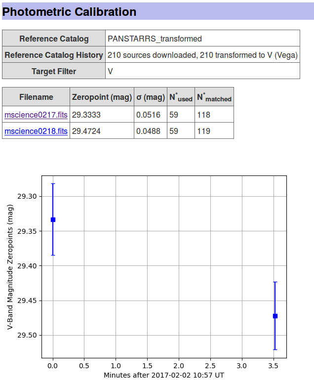
Variations in the magnitude zeropoint are due to changes in the airmass, as well as due to transparency and seeing variations (see FWHM plot above).

In addition to the overview plot, PP provides detailed information on the respective frame page as shown below:

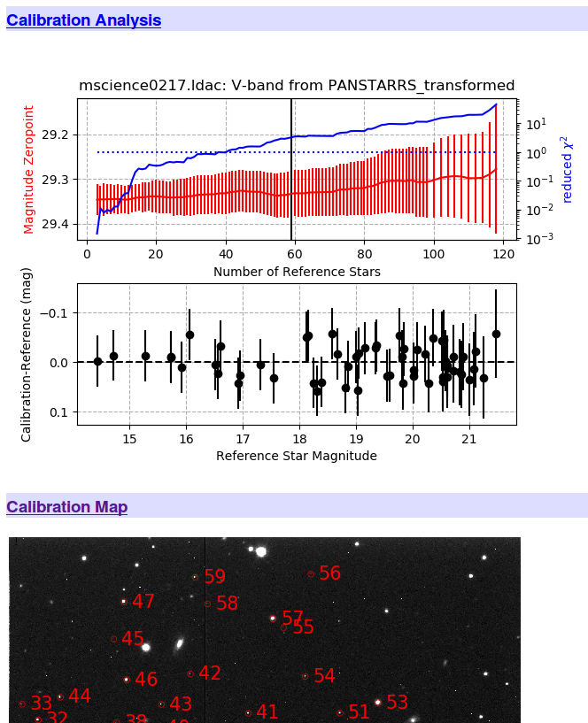
The Calibration Analysis shows the magnitude zeropoint (red line) as a function of the number of background catalog stars used in the calibration. The number of background stars is reduced by rejecting the most significant outlier at a time. The blue line shows the reduced χ:superscript:2 of the remaining data points; the dotted blue line indicates a reduced χ:superscript:2 of 1. Currently, 50% of all background stars are rejected (vertical line) based on their weighted residuals; weights account for photometric uncertainties and catalog uncertainties. This representation shows that the magnitude zeropoint does not depend on the number of background stars used in the calibration. Further options include a Calibration Map, the actual image overplotted with those stars that were used in the final calibration, and the Calibration Data Table listing all background stars used in the final calibration.

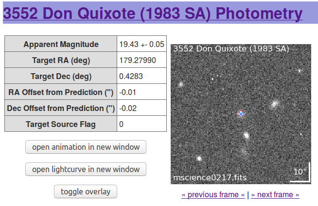
Photometry Results

PP provides final photometry for the actual target(s) in the field, as well as for one reasonably bright star that acts as a Control Star. The Control Star is derived using the exact same calibrations and routines as the target, providing a good verification of the whole process. Usually, the Control Star should have a flat lightcurve that does not show significant variations. However, it cannot be ruled out that the comparison star shows intrinsic variability, or is subject to detector effects, leading to photometric variability. The comparison star is required to be present in the first and the last image of the sequence of images provided.

For each target, PP provides a GIF animation and a lightcurve showing calibrated photometry. The individual frames in the GIF show the expected target position (blue cross) and the actual aperture placement and size used (red circle). The GIF allows for identifying target mismatches and contaminations of the photometry aperture. A is featured for each target, allowing for a quick and easy identification of corrupted frames.

The individual frame page allows for inspecting the corresponding thumbnail image in which the overlay information can deactivated: